[E] Policy Gradients

In this post, we are going to see one of the main approach of reinforcement learning, policy gradients. We will present a step by step proof and derive a useful algorithm. We will also talk about some issues and how to resolve them.

This post assumes some prior knowledge about reinforcement learning. If you have no idea about agent, states, actions, rewards, policy or value functions please check out this blog post first. I have summarized some of the terms in the post but I haven’t described them comprehensively. If you already know what these words mean, we are good to go.

Outline of this post:

• Really Quick Introduction to Reinforcement Learning
• Value Functions
• Policy Gradients
  • Policy Gradient Theorem
• Reducing Variance
  • Reward-to-go
  • Baselines

Really Quick Introduction to Reinforcement Learning

Agent interacts with the environment on different time steps. At every time step \(t\), agent receives the state/observation information and choose an action \(a\) according to its policy \(\pi\) and passes to new state \(s_{t+1}\). After this transaction agent receives a reward signal that denotes how well did the agent perform. (i.e. good action or bad action)

Agents objective is to find actions that maximize the reward on every time step (i.e. cumulative reward).

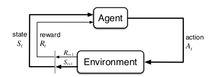
To maximize the reward, there are two main approaches in reinforcement learning. First one is value functions and the second one is policy gradients. Our concern in this article will be on policy gradients.

Value Functions

Before going to deep, let’s briefly introduce the value functions. I believe that even with a small introduction it will help us to understand policy gradients better. Value functions give us the quality of state or state-action pair. State-value function \(V^\pi (s)\) gives us the expected value of being in state \(s\) and then following the policy \(\pi\) afterward. Action-value function \(Q^\pi (s)\) gives us the expected value of being in state \(s\), taking an action \(a\) and then following the policy \(\pi\) afterward. There is a close relation between these two functions: \(V^\pi (s) = \max_a Q^\pi (s)\).

After learning the value functions it’s easy to derive policy by acting greedily in the environment.

This sentence is kind of important to understand the main difference between the value functions and the policy gradients. In value functions, we first learn the value function and derive the policy later. But in policy gradient algorithms we directly learn/optimize the policy.

Policy Gradients

Let’s recall the definition of policy. The policy is a function that maps state \(s\) to action \(a\). It means that we will give the state/observation information to the policy and hopefully, it will return the best action that we should take. In other words, a policy is the brain of an agent.

In the previous section, we mentioned that in policy gradient methods, we directly optimize the policy. We represent our policy with a parameterized function respect to \(\theta\), \(\pi_{\theta} (a \mid s)\), and our objective is to find the best parameters. Let’s write the objective function in a formal way:

where \(r(\tau) = \sum_{t=1}^T r(s_t, a_t)\). As you can see, an objective function depends on the policy. We are trying to find the best parameters \(\theta\) that will return the maximum reward. We can think \(\theta\) as our neural networks parameters/weights. According to the definition of expectation, we can write this objective function in an integral way.

We want the gradient of \(\theta\) respect to \(J(\theta)\). This is the essence of this algorithm. But we cannot directly compute this gradient. Because it contains some terms that we don’t even know. We will apply some transformations and at the end, we will have a useful algorithm. Before going further, let’s define the first term inside the integral and see why we cannot directly compute. It is simply a trajectory probability.

Here \(p(s_1)\) is the initial state distribution. This term is given by the model of the environment. \(\pi_\theta (a_t \mid s_t)\) is our policy at time step \(t\). We completely have control over that thing(i.e. it’s neural network). \(p(s_{t+1} \mid s_t, a_t)\) is transition probability. This term is also given by the model of the environment. Most of the time we don’t know the model of the environment. As a result, we don’t know the transaction probabilities. The reason that we cannot compute gradient is about transaction probabilities. But for a practical algorithm, we don’t need to know it. In the next section, we will see why we don’t need it.

Policy Gradient Theorem

Now hopefully we have a clear setup. We want to calculate the gradient of objective function respect to \(\theta\) and we can not directly compute this gradient. So we have to apply some transformations.

The first thing we are going to do is to put the gradient inside the integral.

\(\nabla_\theta \pi_\theta(\tau)\) this term is difficult to compute. As we saw in the previous section, \(\pi_\theta(\tau)\) includes lots of terms that we don’t know. But there is a convenient algebraic identity that can help us to figure out this gradient.

It’s also called log-derivative trick. This just come froms the derivative of the logarithm. So \(\nabla_\theta \pi_\theta(\tau)\) becomes:

And this is very useful for deriving the policy gradient. Now we can substitute the right-hand side of the above equation(identity) into our integral.

And when we look at this integral, it is an expectation under \(\pi_\theta(\tau)\). It’s some quantity multiplied by \(\pi_\theta(\tau)\) and we integrate over all possible trajectories. That means we can put the expectation back.

So just like our objective as an expectation of \(r(\tau)\), our gradient is an expectation of \(r(\tau)\) \(\nabla_\theta \log{\pi_\theta (\tau)}\)

Now the gradient that we want compute is also an expectation. We need to figure out what \(\nabla_\theta \log{\pi_\theta (\tau)}\) this term is. Let’s rewrite \(\pi_\theta (\tau)\) :

\(\tau\) is shorthand for the sequence of states and actions \(s_1, a_1, s_2, a_2\) etc. until the \(s_T, a_T\). We are interested in the logarithm of this term, so we take the logarithm of both side.

Remember that when take a logarithm of multiplication it turns to summation. Now we need the gradient of this equation. The important thing to note in this huge summation, very few things actually depend on \(\theta\). So initial state distribution \(\log p(s_1)\) is not affected by \(\theta\). It’s derivate w.r.t \(\theta\) is 0. \(\log p(s_{t+1} \mid s_t, a_t)\) the transition probability is also not affected by \(\theta\), so it’s derivative is also 0. If we substitute the remaining term:

We get our policy gradient equation. We said earlier that we don’t need to know the transition probabilities and here is the reason. In this equation there is nothing about transition probabilities. Also, we can compute these terms. Because we only need our policy. Even though we don’t know transition probabilities, we know our policy. Our policy is just a neural network.

But there is one more problem that we need to address. The expectation cannot be computed exactly because the random variable here is extremely high dimensional. We can solve this problem by sampling trajectories in the environment. Then we can use those samples to estimate our gradient.

We will generate samples. For each sample, we will compute its total reward which will give us the second term, and we will also compute the sum of the \(\nabla_\theta \log \pi_\theta (a_{i, t} \mid s_{i, t})\) along that sample which will give us the first term. And once we have estimated this gradient, we will improve our policy with gradient ascent.

And any other stochastic gradient algorithms like Adam, Momentum etc. can be applied to here as well. This procedure has other names as well like REINFORCE algorithm. What we have covered so far gives us the basics of this algorithm.

REINFORCE:

1. Sample trajectories {\(\tau^i\)} from policy \(\pi_{\theta} (a_t \mid s_t)\) (run the policy)
2. Estimate the gradient. \(\nabla_\theta J(\theta) \approx \sum_i \big(\sum_t \nabla_\theta \log \pi_\theta (a_{t}^i \mid s_{t}^i)\big) \big( \sum_{t} r(s_{t}^i, a_{t}^i \big)\)
3. Gradient ascent step. \(\theta \leftarrow \theta + a \nabla_\theta J(\theta)\)

So this is the useful algorithm that we can use. But this version works poorly in practice due to high variance problem. Let’s address this issue in the next section.

Reducing Variance

In this section, we are going to show two tricks to reduce variance of policy gradient algorithms.

Reward To Go

Let’s rewrite the policy gradient algorithm.

In this equation, we punish/reward the agent by the rewards that ever obtained. But it doesn’t make sense because agents should be responsible only for their current actions. This idea of rewarding is called “reward-to-go” and can be expressed like this:

Note that the sum of rewards goes from \(t\) to \(T\). Basic intuition behind this idea is that, if we use less element to calculate variance we will have less variance.

Baselines

The intuition behind the policy gradient is that take the good stuff and make it more likely; take the bad stuff and make it less likely. At first, it seems intuitive but what if all rewards that we get is positive. The plain version of policy gradient will try to boost the probabilities of all actions that return positive reward. Instead of doing that we will introduce a new term called baseline and we will subtract it from the reward:

where \(b = \frac{1}{N} \sum_{i=1}^N r(\tau)\) is the average reward. By introducing baseline, we are saying that increase the probability of actions that is better than average and decrease the probability of actions that is worse than the average. But you may ask that can we really just add or subtract anything from this equation without any trouble? In fact YES. Let’s show that any choice of \(b\) has no effect on the gradient.

If we distribute \(\nabla_\theta \log \pi_\theta (\tau)\) over \(r(\tau) - b\) in expectation we get \(E[\nabla_\theta \log \pi_\theta (\tau) b]\) equals to 0.

Log Derivative Trick: \(\pi_\theta (\tau) \nabla_\theta \log \pi_\theta(\tau) = \nabla_\theta \pi_\theta(\tau)\)

Let’s explain what is going there. In the first line, using the definition of expectation we wrote our equation as an integral. Then we used log-derivative trick again but this time inversely. Then we take the \(b\) and \(\nabla_\theta\) outside of integral. Our policy is a probability distribution over actions so it’s integral is equal to 1. After that, we left with \(b\nabla_\theta 1\) and derivative of 1 is equal to 0. So this whole thing comes out to be 0. That means we can choose any b and add or subtract it from reward, we get the same answer in expectation. But for a finite sample of samples, we don’t get the same variance. And this is really nice because if we choose \(b\) cleverly, we can minimize our variance without changing the expectation.

The most common choice for \(b\) is value function \(V^\pi (s)\).

We represent the value function with the neural network again and update its parameters concurrently with policy function. Our implementation includes both reward to go and neural network baselines. Lastly, I have trained two agents on CartPole and InvertedPendulum environments. Here we show two graphs. The left one is the agent’s learning performance on CartPole environment. Since this environment is pretty easy, using reward-to-go or baseline trick doesn’t make too much difference. But the graph on the right shows a much more clear effect about two tricks. As you can see, the training without reward-to-go and baselines trick is not even close to the optimal. But if we add reward-to-go or baselines we obtain a clear advantage. The red line on the right uses both reward-to-go and baselines trick. As you can see it’s the first network which reaches an optimum.

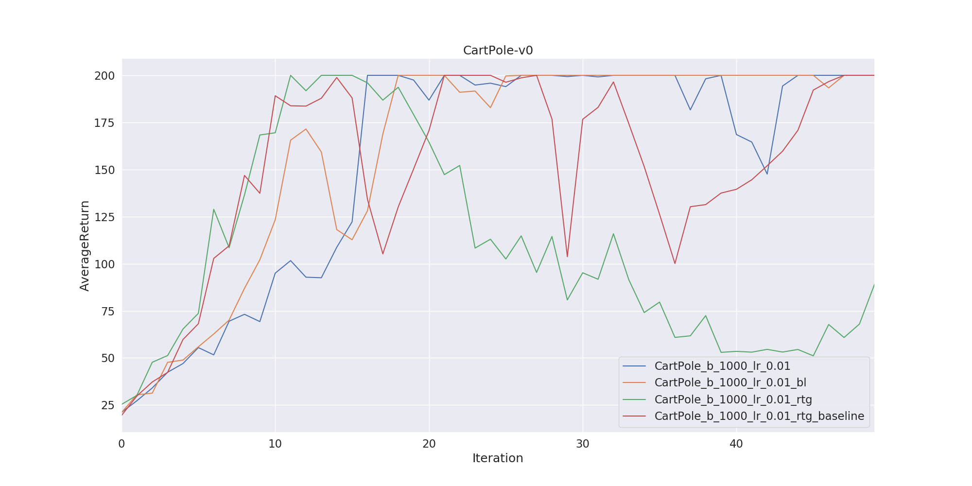
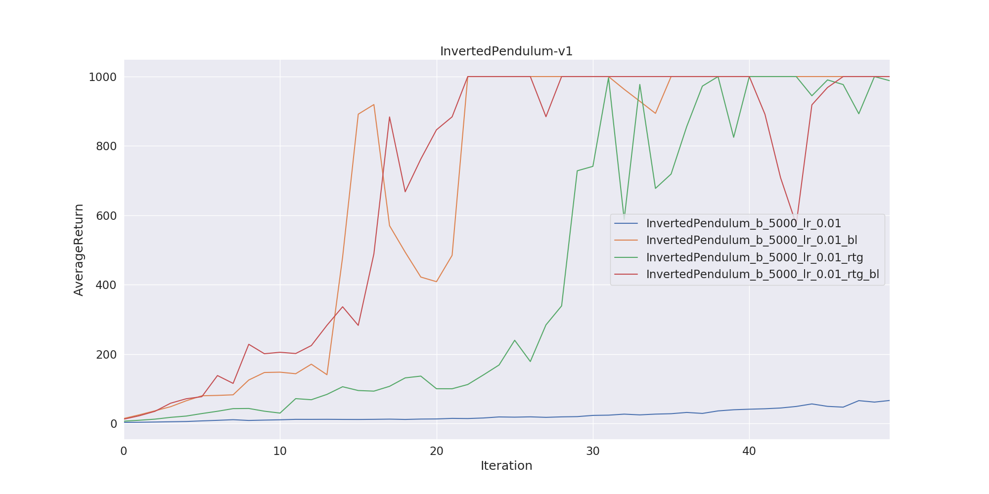
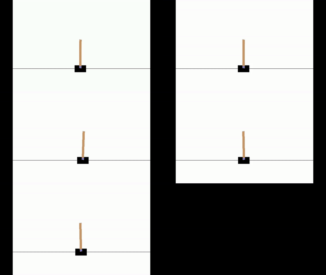
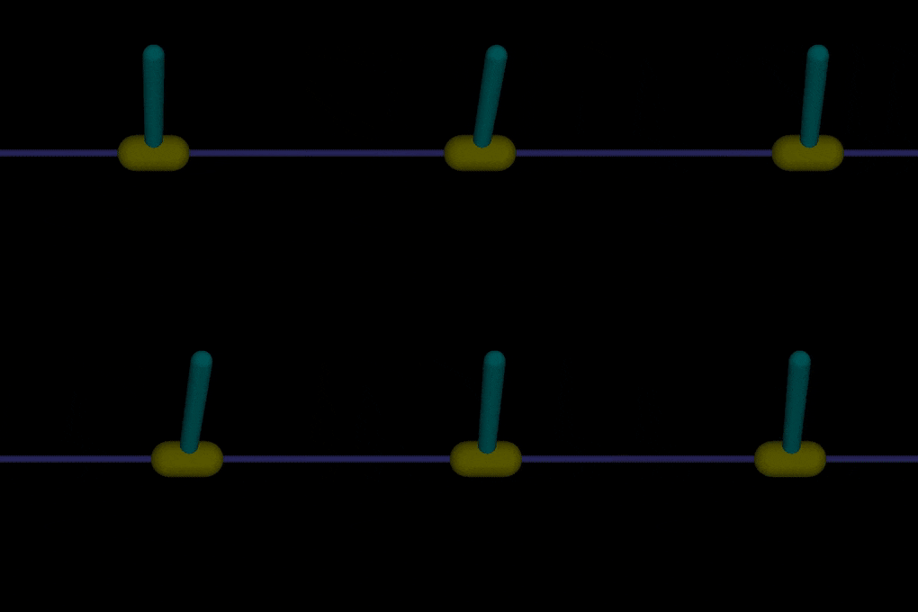
Here’s some agents after training. Respectively, CartPole-v0, LunarLander-v2, InvertedPendulum-v1

Code for this post can be found here.

And that’s it. I tried to explain policy gradients as clear as possible. Please leave a comment if anything is unclear or wrong.

References

[1] Reinforcement Learning: An Introduction 2nd Edition

[2] Berkeley Lecture on Policy Gradients Slide Video

[3] David Silver’s Lecture on Policy Gradients Slide Video

[4] Blog Post by Lilian Weng on Policy Gradient Algorithms